19  Comparison of TransPropy with Other Tool Packages Using CircosBar

library(readr)
library(TransProR)
library(dplyr)
library(rlang)
library(linkET)
library(funkyheatmap)
library(tidyverse)
library(RColorBrewer)
library(ggalluvial)
library(tidyr)
library(tibble)
library(ggplot2)
library(ggridges)
library(GSVA)
library(fgsea) 
library(clusterProfiler)
library(enrichplot)
library(MetaTrx)
library(GseaVis)
library(stringr)
library(cowplot)
library(ggfun)

19.1 select data

# Example: Process the core enrichment genes from TransPropy_CFD_hallmarks_y
TransPropy_CFD_hallmarks_core_enrichment <- TransPropy_CFD_hallmarks_y@result[["core_enrichment"]]
process_core_enrichment(TransPropy_CFD_hallmarks_core_enrichment, correlation_TransPropy_CFD)

# Process the core enrichment genes from deseq2_CFD_hallmarks_y
deseq2_CFD_hallmarks_core_enrichment <- deseq2_CFD_hallmarks_y@result[["core_enrichment"]]
process_core_enrichment(deseq2_CFD_hallmarks_core_enrichment, correlation_deseq2_CFD)

# Process the core enrichment genes from edgeR_CFD_hallmarks_y
edgeR_CFD_hallmarks_core_enrichment <- edgeR_CFD_hallmarks_y@result[["core_enrichment"]]
process_core_enrichment(edgeR_CFD_hallmarks_core_enrichment, correlation_edgeR_CFD)

# Process the core enrichment genes from limma_CFD_hallmarks_y
limma_CFD_hallmarks_core_enrichment <- limma_CFD_hallmarks_y@result[["core_enrichment"]]
process_core_enrichment(limma_CFD_hallmarks_core_enrichment, correlation_limma_CFD)

# Process the core enrichment genes from outRst_CFD_hallmarks_y
outRst_CFD_hallmarks_core_enrichment <- outRst_CFD_hallmarks_y@result[["core_enrichment"]]
process_core_enrichment(outRst_CFD_hallmarks_core_enrichment, correlation_outRst_CFD)




# Process the core enrichment genes from TransPropy_CFD_kegg_y
TransPropy_CFD_kegg_core_enrichment <- TransPropy_CFD_kegg_y@result[["core_enrichment"]]
process_core_enrichment(TransPropy_CFD_kegg_core_enrichment, correlation_TransPropy_CFD)

# Process the core enrichment genes from deseq2_CFD_kegg_y
deseq2_CFD_kegg_core_enrichment <- deseq2_CFD_kegg_y@result[["core_enrichment"]]
process_core_enrichment(deseq2_CFD_kegg_core_enrichment, correlation_deseq2_CFD)

# Process the core enrichment genes from edgeR_CFD_kegg_y
edgeR_CFD_kegg_core_enrichment <- edgeR_CFD_kegg_y@result[["core_enrichment"]]
process_core_enrichment(edgeR_CFD_kegg_core_enrichment, correlation_edgeR_CFD)

# Process the core enrichment genes from limma_CFD_kegg_y
limma_CFD_kegg_core_enrichment <- limma_CFD_kegg_y@result[["core_enrichment"]]
process_core_enrichment(limma_CFD_kegg_core_enrichment, correlation_limma_CFD)

# Process the core enrichment genes from outRst_CFD_kegg_y
outRst_CFD_kegg_core_enrichment <- outRst_CFD_kegg_y@result[["core_enrichment"]]
process_core_enrichment(outRst_CFD_kegg_core_enrichment, correlation_outRst_CFD)




# Process the core enrichment genes from TransPropy_ANKRD35_hallmarks_y
TransPropy_ANKRD35_hallmarks_core_enrichment <- TransPropy_ANKRD35_hallmarks_y@result[["core_enrichment"]]
process_core_enrichment(TransPropy_ANKRD35_hallmarks_core_enrichment, correlation_TransPropy_ANKRD35)

# Process the core enrichment genes from deseq2_ANKRD35_hallmarks_y
deseq2_ANKRD35_hallmarks_core_enrichment <- deseq2_ANKRD35_hallmarks_y@result[["core_enrichment"]]
process_core_enrichment(deseq2_ANKRD35_hallmarks_core_enrichment, correlation_deseq2_ANKRD35)

# Process the core enrichment genes from edgeR_ANKRD35_hallmarks_y
edgeR_ANKRD35_hallmarks_core_enrichment <- edgeR_ANKRD35_hallmarks_y@result[["core_enrichment"]]
process_core_enrichment(edgeR_ANKRD35_hallmarks_core_enrichment, correlation_edgeR_ANKRD35)

# Process the core enrichment genes from limma_ANKRD35_hallmarks_y
limma_ANKRD35_hallmarks_core_enrichment <- limma_ANKRD35_hallmarks_y@result[["core_enrichment"]]
process_core_enrichment(limma_ANKRD35_hallmarks_core_enrichment, correlation_limma_ANKRD35)

# Process the core enrichment genes from outRst_ANKRD35_hallmarks_y
outRst_ANKRD35_hallmarks_core_enrichment <- outRst_ANKRD35_hallmarks_y@result[["core_enrichment"]]
process_core_enrichment(outRst_ANKRD35_hallmarks_core_enrichment, correlation_outRst_ANKRD35)




# Process the core enrichment genes from TransPropy_ANKRD35_kegg_y
TransPropy_ANKRD35_kegg_core_enrichment <- TransPropy_ANKRD35_kegg_y@result[["core_enrichment"]]
process_core_enrichment(TransPropy_ANKRD35_kegg_core_enrichment, correlation_TransPropy_ANKRD35)

# Process the core enrichment genes from deseq2_ANKRD35_kegg_y
deseq2_ANKRD35_kegg_core_enrichment <- deseq2_ANKRD35_kegg_y@result[["core_enrichment"]]
process_core_enrichment(deseq2_ANKRD35_kegg_core_enrichment, correlation_deseq2_ANKRD35)

# Process the core enrichment genes from edgeR_ANKRD35_kegg_y
edgeR_ANKRD35_kegg_core_enrichment <- edgeR_ANKRD35_kegg_y@result[["core_enrichment"]]
process_core_enrichment(edgeR_ANKRD35_kegg_core_enrichment, correlation_edgeR_ANKRD35)

# Process the core enrichment genes from limma_ANKRD35_kegg_y
limma_ANKRD35_kegg_core_enrichment <- limma_ANKRD35_kegg_y@result[["core_enrichment"]]
process_core_enrichment(limma_ANKRD35_kegg_core_enrichment, correlation_limma_ANKRD35)

# Process the core enrichment genes from outRst_ANKRD35_kegg_y
outRst_ANKRD35_kegg_core_enrichment <- outRst_ANKRD35_kegg_y@result[["core_enrichment"]]
process_core_enrichment(outRst_ANKRD35_kegg_core_enrichment, correlation_outRst_ANKRD35)




# Process the core enrichment genes from TransPropy_ALOXE3_hallmarks_y
TransPropy_ALOXE3_hallmarks_core_enrichment <- TransPropy_ALOXE3_hallmarks_y@result[["core_enrichment"]]
process_core_enrichment(TransPropy_ALOXE3_hallmarks_core_enrichment, correlation_TransPropy_ALOXE3)

# Process the core enrichment genes from deseq2_ALOXE3_hallmarks_y
deseq2_ALOXE3_hallmarks_core_enrichment <- deseq2_ALOXE3_hallmarks_y@result[["core_enrichment"]]
process_core_enrichment(deseq2_ALOXE3_hallmarks_core_enrichment, correlation_deseq2_ALOXE3)

# Process the core enrichment genes from edgeR_ALOXE3_hallmarks_y
edgeR_ALOXE3_hallmarks_core_enrichment <- edgeR_ALOXE3_hallmarks_y@result[["core_enrichment"]]
process_core_enrichment(edgeR_ALOXE3_hallmarks_core_enrichment, correlation_edgeR_ALOXE3)

# Process the core enrichment genes from limma_ALOXE3_hallmarks_y
limma_ALOXE3_hallmarks_core_enrichment <- limma_ALOXE3_hallmarks_y@result[["core_enrichment"]]
process_core_enrichment(limma_ALOXE3_hallmarks_core_enrichment, correlation_limma_ALOXE3)

# Process the core enrichment genes from outRst_ALOXE3_hallmarks_y
outRst_ALOXE3_hallmarks_core_enrichment <- outRst_ALOXE3_hallmarks_y@result[["core_enrichment"]]
process_core_enrichment(outRst_ALOXE3_hallmarks_core_enrichment, correlation_outRst_ALOXE3)




# Process the core enrichment genes from TransPropy_ALOXE3_kegg_y
TransPropy_ALOXE3_kegg_core_enrichment <- TransPropy_ALOXE3_kegg_y@result[["core_enrichment"]]
process_core_enrichment(TransPropy_ALOXE3_kegg_core_enrichment, correlation_TransPropy_ALOXE3)

# Process the core enrichment genes from deseq2_ALOXE3_kegg_y
deseq2_ALOXE3_kegg_core_enrichment <- deseq2_ALOXE3_kegg_y@result[["core_enrichment"]]
process_core_enrichment(deseq2_ALOXE3_kegg_core_enrichment, correlation_deseq2_ALOXE3)

# Process the core enrichment genes from edgeR_ALOXE3_kegg_y
edgeR_ALOXE3_kegg_core_enrichment <- edgeR_ALOXE3_kegg_y@result[["core_enrichment"]]
process_core_enrichment(edgeR_ALOXE3_kegg_core_enrichment, correlation_edgeR_ALOXE3)

# Process the core enrichment genes from limma_ALOXE3_kegg_y
limma_ALOXE3_kegg_core_enrichment <- limma_ALOXE3_kegg_y@result[["core_enrichment"]]
process_core_enrichment(limma_ALOXE3_kegg_core_enrichment, correlation_limma_ALOXE3)

# Process the core enrichment genes from outRst_ALOXE3_kegg_y
outRst_ALOXE3_kegg_core_enrichment <- outRst_ALOXE3_kegg_y@result[["core_enrichment"]]
process_core_enrichment(outRst_ALOXE3_kegg_core_enrichment, correlation_outRst_ALOXE3)

19.2 data

barcircosdata = tribble(
  ~Gene,    ~Pathway,   ~Methods, ~type, ~Pos_Neg, ~count,
  
  "CFD",  "hallmarks","deseq2", "unique","positive",61,
  "CFD",  "hallmarks","deseq2", "unique","negative",21,
  "CFD",  "hallmarks","deseq2", "notunique","positive",79,
  "CFD",  "hallmarks","deseq2", "notunique","negative",21,
  "CFD",  "hallmarks","edgeR","unique","positive",43,
  "CFD",  "hallmarks","edgeR","unique","negative",21,
  "CFD",  "hallmarks","edgeR","notunique","positive",52,
  "CFD",  "hallmarks","edgeR","notunique","negative",21,
  "CFD",  "hallmarks","TransPropy","unique", "positive",45,
  "CFD",  "hallmarks","TransPropy","unique", "negative",74,
  "CFD",  "hallmarks","TransPropy","notunique","positive",48,
  "CFD",  "hallmarks","TransPropy","notunique","negative",102,
  "CFD",  "hallmarks","limma","unique","positive",84,
  "CFD",  "hallmarks","limma","unique","negative",143,
  "CFD",  "hallmarks","limma","notunique","positive",93,
  "CFD",  "hallmarks","limma","notunique","negative",213,
  "CFD",  "hallmarks","outRst","unique","positive",37,
  "CFD",  "hallmarks","outRst","unique","negative",97,
  "CFD",  "hallmarks","outRst","notunique","positive",38,
  "CFD",  "hallmarks","outRst","notunique","negative",150,
  

  "CFD",  "kegg","deseq2", "unique","positive",38,
  "CFD",  "kegg","deseq2", "unique","negative",0,
  "CFD",  "kegg","deseq2", "notunique","positive",83,
  "CFD",  "kegg","deseq2", "notunique","negative",0,
  "CFD",  "kegg","edgeR","unique","positive",28,
  "CFD",  "kegg","edgeR","unique","negative",0,
  "CFD",  "kegg","edgeR","notunique","positive",53,
  "CFD",  "kegg","edgeR","notunique","negative",0,
  "CFD",  "kegg","TransPropy","unique", "positive",51,
  "CFD",  "kegg","TransPropy","unique", "negative",23,
  "CFD",  "kegg","TransPropy","notunique","positive",94,
  "CFD",  "kegg","TransPropy","notunique","negative",23,
  "CFD",  "kegg","limma","unique","positive",31,
  "CFD",  "kegg","limma","unique","negative",77,
  "CFD",  "kegg","limma","notunique","positive",41,
  "CFD",  "kegg","limma","notunique","negative",152,
  "CFD",  "kegg","outRst","unique","positive",24,
  "CFD",  "kegg","outRst","unique","negative",81,
  "CFD",  "kegg","outRst","notunique","positive",31,
  "CFD",  "kegg","outRst","notunique","negative",179,
  
  
  
  
  "ANKRD35",  "hallmarks","deseq2", "unique","positive",62,
  "ANKRD35",  "hallmarks","deseq2", "unique","negative",21,
  "ANKRD35",  "hallmarks","deseq2", "notunique","positive",84,
  "ANKRD35",  "hallmarks","deseq2", "notunique","negative",21,
  "ANKRD35",  "hallmarks","edgeR","unique","positive",43,
  "ANKRD35",  "hallmarks","edgeR","unique","negative",21,
  "ANKRD35",  "hallmarks","edgeR","notunique","positive",52,
  "ANKRD35",  "hallmarks","edgeR","notunique","negative",21,
  "ANKRD35",  "hallmarks","TransPropy","unique", "positive",59,
  "ANKRD35",  "hallmarks","TransPropy","unique", "negative",87,
  "ANKRD35",  "hallmarks","TransPropy","notunique","positive",67,
  "ANKRD35",  "hallmarks","TransPropy","notunique","negative",119,
  "ANKRD35",  "hallmarks","limma","unique","positive",108,
  "ANKRD35",  "hallmarks","limma","unique","negative",153,
  "ANKRD35",  "hallmarks","limma","notunique","positive",135,
  "ANKRD35",  "hallmarks","limma","notunique","negative",231,
  "ANKRD35",  "hallmarks","outRst","unique","positive",56,
  "ANKRD35",  "hallmarks","outRst","unique","negative",101,
  "ANKRD35",  "hallmarks","outRst","notunique","positive",71,
  "ANKRD35",  "hallmarks","outRst","notunique","negative",160,
  
  

  "ANKRD35",  "kegg","deseq2", "unique","positive",42,
  "ANKRD35",  "kegg","deseq2", "unique","negative",14,
  "ANKRD35",  "kegg","deseq2", "notunique","positive",91,
  "ANKRD35",  "kegg","deseq2", "notunique","negative",14,
  "ANKRD35",  "kegg","edgeR","unique","positive",29,
  "ANKRD35",  "kegg","edgeR","unique","negative",0,
  "ANKRD35",  "kegg","edgeR","notunique","positive",72,
  "ANKRD35",  "kegg","edgeR","notunique","negative",0,
  "ANKRD35",  "kegg","TransPropy","unique", "positive",53,
  "ANKRD35",  "kegg","TransPropy","unique", "negative",42,
  "ANKRD35",  "kegg","TransPropy","notunique","positive",97,
  "ANKRD35",  "kegg","TransPropy","notunique","negative",63,
  "ANKRD35",  "kegg","limma","unique","positive",40,
  "ANKRD35",  "kegg","limma","unique","negative",105,
  "ANKRD35",  "kegg","limma","notunique","positive",74,
  "ANKRD35",  "kegg","limma","notunique","negative",246,
  "ANKRD35",  "kegg","outRst","unique","positive",22,
  "ANKRD35",  "kegg","outRst","unique","negative",81,
  "ANKRD35",  "kegg","outRst","notunique","positive",27,
  "ANKRD35",  "kegg","outRst","notunique","negative",192,
  
  
  

  "ALOXE3",  "hallmarks","deseq2", "unique","positive",65,
  "ALOXE3",  "hallmarks","deseq2", "unique","negative",21,
  "ALOXE3",  "hallmarks","deseq2", "notunique","positive",87,
  "ALOXE3",  "hallmarks","deseq2", "notunique","negative",21,
  "ALOXE3",  "hallmarks","edgeR","unique","positive",41,
  "ALOXE3",  "hallmarks","edgeR","unique","negative",0,
  "ALOXE3",  "hallmarks","edgeR","notunique","positive",49,
  "ALOXE3",  "hallmarks","edgeR","notunique","negative",0,
  "ALOXE3",  "hallmarks","TransPropy","unique", "positive",71,
  "ALOXE3",  "hallmarks","TransPropy","unique", "negative",104,
  "ALOXE3",  "hallmarks","TransPropy","notunique","positive",85,
  "ALOXE3",  "hallmarks","TransPropy","notunique","negative",141,
  "ALOXE3",  "hallmarks","limma","unique","positive",96,
  "ALOXE3",  "hallmarks","limma","unique","negative",139,
  "ALOXE3",  "hallmarks","limma","notunique","positive",119,
  "ALOXE3",  "hallmarks","limma","notunique","negative",204,
  "ALOXE3",  "hallmarks","outRst","unique","positive",73,
  "ALOXE3",  "hallmarks","outRst","unique","negative",101,
  "ALOXE3",  "hallmarks","outRst","notunique","positive",91,
  "ALOXE3",  "hallmarks","outRst","notunique","negative",161,
  
  
  
  

  "ALOXE3",  "kegg","deseq2", "unique","positive",51,
  "ALOXE3",  "kegg","deseq2", "unique","negative",0,
  "ALOXE3",  "kegg","deseq2", "notunique","positive",115,
  "ALOXE3",  "kegg","deseq2", "notunique","negative",0,
  "ALOXE3",  "kegg","edgeR","unique","positive",31,
  "ALOXE3",  "kegg","edgeR","unique","negative",0,
  "ALOXE3",  "kegg","edgeR","notunique","positive",77,
  "ALOXE3",  "kegg","edgeR","notunique","negative",0,
  "ALOXE3",  "kegg","TransPropy","unique", "positive",48,
  "ALOXE3",  "kegg","TransPropy","unique", "negative",27,
  "ALOXE3",  "kegg","TransPropy","notunique","positive",86,
  "ALOXE3",  "kegg","TransPropy","notunique","negative",27,
  "ALOXE3",  "kegg","limma","unique","positive",20,
  "ALOXE3",  "kegg","limma","unique","negative",50,
  "ALOXE3",  "kegg","limma","notunique","positive",28,
  "ALOXE3",  "kegg","limma","notunique","negative",124,
  "ALOXE3",  "kegg","outRst","unique","positive",53,
  "ALOXE3",  "kegg","outRst","unique","negative",85,
  "ALOXE3",  "kegg","outRst","notunique","positive",82,
  "ALOXE3",  "kegg","outRst","notunique","negative",198
  
)

19.3 first image

barcircosdata$Kind5 <-1

# Create a factor for Gene in the order of its appearance
barcircosdata$Gene <- factor(barcircosdata$Gene, levels = unique(barcircosdata$Gene))


test_df2 <- barcircosdata %>%
  dplyr::mutate(Pathway = str_c(Gene, Pathway, sep = "_")) %>%
  dplyr::mutate(Methods = str_c(Pathway, Methods, sep = "_")) %>%
  dplyr::mutate(type = str_c(Methods, type, sep = "_"))

# Kind3
# Ensure that the order of type remains consistent throughout the process and apply angle calculations correctly. It may be necessary to further check and adjust the logic of the code.
# To ensure the correct order, explicitly set factor levels and sort the data before calculating angles.
# Otherwise, the order of type in test_df_Kind4 and test_df2 may differ, causing mapping issues in subsequent plots.
# Ensure the type column is a factor and ordered as needed
test_df2 <- test_df2 %>%
  mutate(Methods = factor(Methods, levels = unique(Methods)))

test_df_Kind3 <- test_df2 %>%
  group_by(Methods) %>%
  summarise(sum_Kind = sum(Kind5), .groups = 'drop') %>%
  mutate(cumsum_Kind = cumsum(sum_Kind),
          total_Kind = sum(sum_Kind),
          id = row_number(),  # Compute a unique row number for each Methods
         angle = 90 - 360 * (id - 0.5) / n(),  # Use a new angle calculation formula
          hjust = ifelse(angle < -90, 0.5, 0.5),
          label_position = ifelse(angle > -90, angle + 180, angle))  # Adjust angles

# Ensure that the order of type remains consistent throughout the process and apply angle calculations correctly. It may be necessary to further check and adjust the logic of the code.
# To ensure the correct order, explicitly set factor levels and sort the data before calculating angles.
# Otherwise, the order of type in test_df_Kind4 and test_df2 may differ, causing mapping issues in subsequent plots.
# Ensure the type column is a factor and ordered as needed
test_df2 <- test_df2 %>%
  mutate(type = factor(type, levels = unique(type)))

# Kind4
test_df_Kind4 <- test_df2 %>%
  group_by(type) %>%
  summarise(sum_Kind = sum(Kind5), .groups = 'drop') %>%
  arrange(type) %>%  # Sort by type
  mutate(cumsum_Kind = cumsum(sum_Kind),
          total_Kind = sum(sum_Kind),
          id = row_number(),  # Compute a unique row number for each type
         angle = 90 - 360 * (id - 0.5) / n(),  # Use a new angle calculation formula
          hjust = ifelse(angle < -90, 0.5, 0.5),
          label_position = ifelse(angle > -90, angle + 180, angle))  # Adjust angles

ggplot(data = test_df2) + 
  # Kind
  geom_col(data = test_df2 %>%
             dplyr::group_by(Gene) %>%
             dplyr::summarise(sum_Kind = sum(Kind5)),
           aes(x = 0, y = sum_Kind, fill = Gene), fill = "#863630", color = "#ffffff", width = 1, alpha = 0.9) + 
  geom_text(data = test_df2 %>%
              dplyr::select(Gene, Kind5) %>%
              dplyr::group_by(Gene) %>%
              dplyr::summarise(sum_Kind = sum(Kind5)) %>%
              dplyr::mutate(cumsum_Kind = cumsum(sum_Kind),
                            id = 1:nrow(.)),
            aes(x = 0, y = cumsum_Kind - 0.5 * sum_Kind, label = Gene),
            angle = c(-60, 0, 60),
            vjust = c(0.5, 0.5, 0.5),
            color = "#000000",
            size = 4
  ) + 
  # Kind2
  geom_col(data = test_df2 %>%
             dplyr::group_by(Pathway) %>%
             dplyr::summarise(sum_Kind2 = sum(Kind5)),
           aes(x = 1, y = sum_Kind2, fill = Pathway), fill = "#f57918", color = "#ffffff", width = 1, alpha = 0.9) +
  geom_text(data = test_df2 %>%
              dplyr::select(Pathway, Kind5) %>%
              dplyr::group_by(Pathway) %>%
              dplyr::summarise(sum_Kind = sum(Kind5)) %>%
              dplyr::mutate(cumsum_Kind = cumsum(sum_Kind)),
            aes(x = 1, y = cumsum_Kind - 0.5 * sum_Kind, label = str_remove(Pathway, pattern = ".*_")),
            color = "#000000",
            size = 3.5
  ) + 
  # Kind3
  geom_col(data = test_df2 %>%
             dplyr::group_by(Methods) %>%
             dplyr::summarise(sum_Kind3 = sum(Kind5)),
           aes(x = 2, y = sum_Kind3, fill = Methods), fill = "#f5b201", color = "#ffffff", width = 1, alpha = 0.9) + 
  geom_text(data = test_df_Kind3,
            aes(x = 2, y = cumsum_Kind - 0.5 * sum_Kind, label = str_remove(Methods, pattern = ".*_"), hjust=hjust),
            angle= test_df_Kind3$label_position + 180,
            color = "#000000",
            size = 3
  ) + 
  # Kind4
  geom_col(data = test_df2 %>%
             dplyr::group_by(type) %>%
             dplyr::summarise(sum_Kind4 = sum(Kind5)),
           aes(x = 3, y = sum_Kind4, fill = type), fill = "#f4d301", color = "#ffffff", width = 1, alpha = 0.9) + 
  geom_text(data = test_df_Kind4,
            aes(x = 3, y = cumsum_Kind - 0.5 * sum_Kind, label = str_remove(type, pattern = ".*_"), hjust=hjust),
            angle= test_df_Kind4$label_position+ 180,
            color = "#000000",
            size = 3.1
  )+ 
  coord_polar(theta = "y") + 
  theme_nothing() + 
  theme(plot.margin = margin(t = 0.5, r = 0.5, b = 0.5, l = 0.5, unit = "cm"))-> p1

p1

# Merge columns
barcircosdata1 <- barcircosdata %>%
  unite("Name", Gene, Pathway, Methods, type, sep = "_")

# Generate ID column
plot_test_df2 <- barcircosdata1 %>%
  mutate(ID = as.numeric(factor(Name, levels = unique(Name))))

# If IDs are duplicated, angle calculations will indeed be affected, as angles are calculated based on the number of rows (nrow). We can modify the code to ensure that each unique ID has only one angle, instead of calculating the angle for each row. We need to group the data and perform angle calculations.
# We can use distinct to extract unique IDs and calculate angles based on the unique IDs, then merge back to the original dataframe.
# Extract unique IDs and calculate angles
unique_ids <- plot_test_df2 %>%
  distinct(ID) %>%
  arrange(ID) %>%
  mutate(
    angle = 90 - 360 * (ID - 0.5) / n(),
    hjust = ifelse(angle < -90, 1, 0),
    angle2 = ifelse(angle < -90, angle + 180, angle)
  )

# Merge angle information back to the original dataframe
plot_test_df2 <- plot_test_df2 %>%
  left_join(unique_ids, by = "ID")

# Calculate percentage
plot_test_df2 <- plot_test_df2 %>%
  group_by(ID) %>%
  mutate(total = sum(count),
         percentage = (count / total) * 100) %>%
  ungroup()

19.4 second image

# Bar stacking (alternative)

p21 <- ggplot(plot_test_df2, aes(x = as.factor(ID), y = count, fill = Pos_Neg)) +
  geom_bar(position = "stack", color = "#000000", stat = "identity", alpha = 0.9) +
  scale_fill_manual(values = c('#236d18', '#8daf00')) + # Custom color
  geom_text(aes(x = as.factor(ID), y = count + 10, label = count), 
            position = position_stack(vjust = 0), # Ensure each label starts at the beginning of each stacked bar
            color = "#000000", 
            fontface = "bold",
            size = 3, 
            angle = plot_test_df2$angle2, 
            hjust = plot_test_df2$hjust) + 
  ylim(-770, 370) +
  theme_void() +
  theme(
    legend.position = c(0.99, 0.5)
  ) +
  coord_polar(start = 0)

# Print the plot
print(p21)

# Percentage
# Create plot
p21 <- ggplot(plot_test_df2, aes(x = as.factor(ID), y = percentage, fill = Pos_Neg)) +
  geom_bar(position = "stack", color = "#000000", stat = "identity", alpha = 0.9) +
  scale_fill_manual(values = c('#236d18', '#8daf00')) + # Custom color
  geom_text(aes(x = as.factor(ID), y = percentage + 10, label = paste0(round(percentage, 0), "%")), 
            position = position_stack(vjust = 0.1), # Ensure each label is at 0.1 height of each stacked bar
            color = "#000000", 
            fontface = "bold",
            size = 3, 
            angle = plot_test_df2$angle2, 
            hjust = plot_test_df2$hjust) + 
  ylim(-210, 110) +
  theme_void() +
  theme(
    legend.position = c(1, 0.5)
  ) +
  coord_polar(start = 0) +
  # Add the 50% line
  geom_segment(aes(x = 0.5, xend = length(unique(ID)) + 0.5, 
                   y = 50, yend = 50), 
               color = "#e5d87c", size = 1.5, alpha = 0.7)

# Print the plot
print(p21)

19.5 third image

# Create df111 data frame
methods <- rep(c("deseq2", "edgeR", "TransPropy", "limma", "outRst"), times = 6)
# Create df111 data frame
df111 <- data.frame(
  methods = methods,
  ID = 1:length(methods),
  segment = rep(c(rep("hallmarks", times = 5), rep("kegg", times = 5)), times = 3),
  segmentcolors = rep(c("#f5b201", "#f5b201", "#3c7a38", "#f57918", "#f57918"), times = 6)
)
# Add start and end columns to indicate the start and end of each bar
df111$start <- (df111$ID - 1) * 1
df111$end <- df111$ID * 1

# Plot color segments without gaps
p3 <- ggplot(df111) +
  geom_rect(aes(xmin = start, xmax = end, ymin = 0, ymax = 15, fill = segmentcolors), alpha = 0.9) +
  scale_fill_identity() +  # Use identity mapping for colors
  theme_void() +
  theme(axis.text.y = element_blank(), axis.ticks.y = element_blank(), axis.title.y = element_blank()) +
  coord_polar(start = 0) +
  ylim(-200, 50)

# Plot color segments with gaps (alternative)
p3 <- ggplot(df111, aes(x = factor(ID), y = 10, fill = segmentcolors)) +
  geom_col(alpha = 0.9) +
  scale_fill_identity() +  # Use identity mapping for colors
  theme_void() +
  theme(axis.text.y = element_blank(), axis.ticks.y = element_blank(), axis.title.y = element_blank()) +
  coord_polar(start = 0) +
  ylim(-200, 50)

# Display the plot
print(p3)

19.6 Combine plots (percentage)

# Combine plots
p_combine <- ggdraw(p21) + 
  draw_plot(p1, x = 0.15, y = 0.15, width = 0.7, height = 0.7) +
  draw_plot(p3, x = -0.125, y = -0.125, width = 1.25, height = 1.25)

# Display the combined plot
print(p_combine)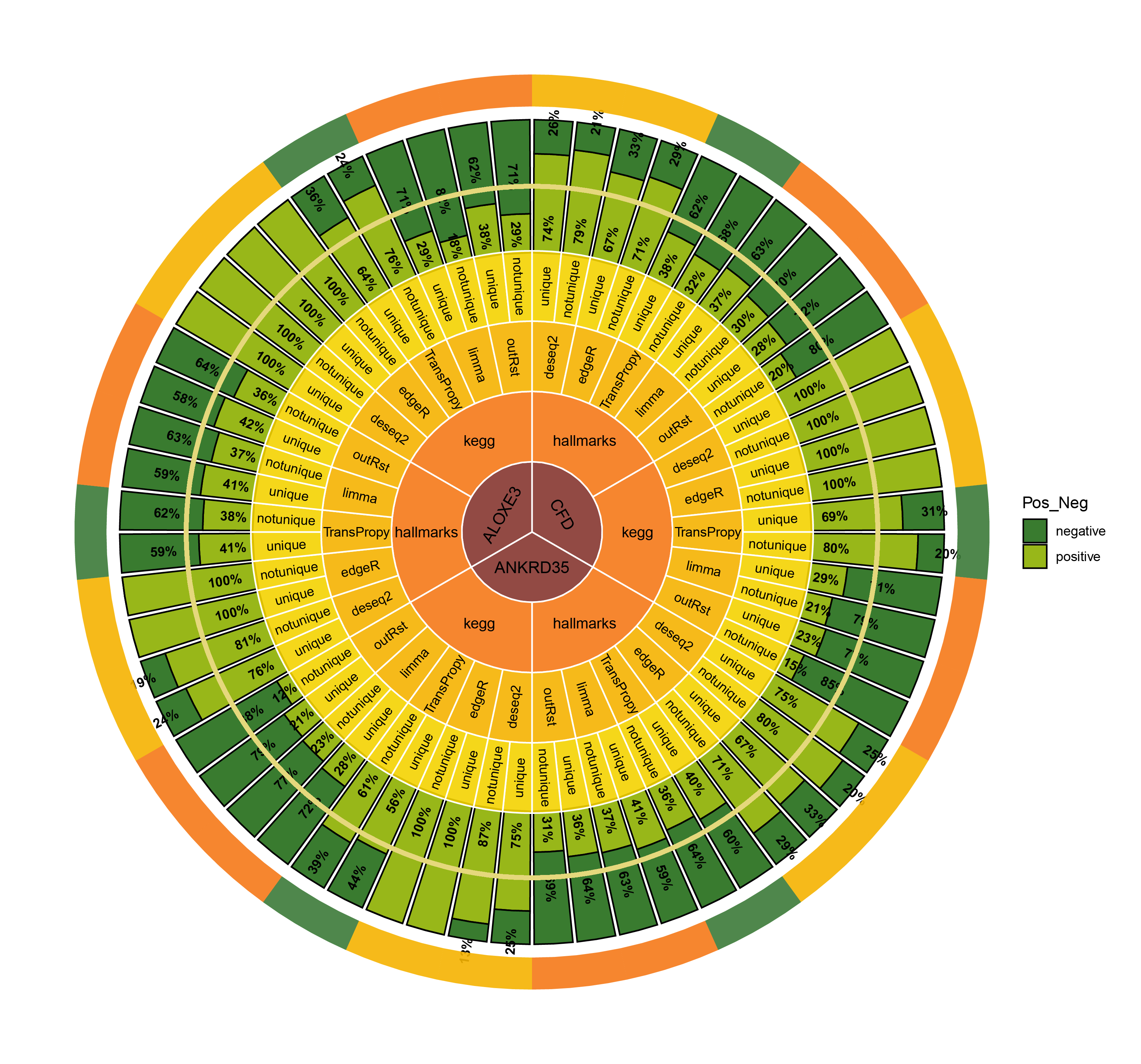

CircosBar core enrichment_percentage

19.7 Combine plots (percentage)

barcircosdata = tribble(
  ~Gene,    ~Pathway,   ~Methods, ~type, ~Pos_Neg, ~count,
  
  "CFD",  "hallmarks","deseq2", "unique","positive",61,
  "CFD",  "hallmarks","deseq2", "unique","negative",21,
  "CFD",  "hallmarks","deseq2", "notunique","positive",79,
  "CFD",  "hallmarks","deseq2", "notunique","negative",21,
  "CFD",  "hallmarks","edgeR","unique","positive",43,
  "CFD",  "hallmarks","edgeR","unique","negative",21,
  "CFD",  "hallmarks","edgeR","notunique","positive",52,
  "CFD",  "hallmarks","edgeR","notunique","negative",21,
  "CFD",  "hallmarks","TransPropy","unique", "positive",45,
  "CFD",  "hallmarks","TransPropy","unique", "negative",74,
  "CFD",  "hallmarks","TransPropy","notunique","positive",48,
  "CFD",  "hallmarks","TransPropy","notunique","negative",102,
  "CFD",  "hallmarks","limma","unique","positive",84,
  "CFD",  "hallmarks","limma","unique","negative",143,
  "CFD",  "hallmarks","limma","notunique","positive",93,
  "CFD",  "hallmarks","limma","notunique","negative",213,
  "CFD",  "hallmarks","outRst","unique","positive",37,
  "CFD",  "hallmarks","outRst","unique","negative",97,
  "CFD",  "hallmarks","outRst","notunique","positive",38,
  "CFD",  "hallmarks","outRst","notunique","negative",150,
  
  
  "CFD",  "kegg","deseq2", "unique","positive",38,
  "CFD",  "kegg","deseq2", "unique","negative",0,
  "CFD",  "kegg","deseq2", "notunique","positive",83,
  "CFD",  "kegg","deseq2", "notunique","negative",0,
  "CFD",  "kegg","edgeR","unique","positive",28,
  "CFD",  "kegg","edgeR","unique","negative",0,
  "CFD",  "kegg","edgeR","notunique","positive",53,
  "CFD",  "kegg","edgeR","notunique","negative",0,
  "CFD",  "kegg","TransPropy","unique", "positive",51,
  "CFD",  "kegg","TransPropy","unique", "negative",23,
  "CFD",  "kegg","TransPropy","notunique","positive",94,
  "CFD",  "kegg","TransPropy","notunique","negative",23,
  "CFD",  "kegg","limma","unique","positive",31,
  "CFD",  "kegg","limma","unique","negative",77,
  "CFD",  "kegg","limma","notunique","positive",41,
  "CFD",  "kegg","limma","notunique","negative",152,
  "CFD",  "kegg","outRst","unique","positive",24,
  "CFD",  "kegg","outRst","unique","negative",81,
  "CFD",  "kegg","outRst","notunique","positive",31,
  "CFD",  "kegg","outRst","notunique","negative",179,
  
  
  
  
  "ANKRD35",  "hallmarks","deseq2", "unique","positive",62,
  "ANKRD35",  "hallmarks","deseq2", "unique","negative",21,
  "ANKRD35",  "hallmarks","deseq2", "notunique","positive",84,
  "ANKRD35",  "hallmarks","deseq2", "notunique","negative",21,
  "ANKRD35",  "hallmarks","edgeR","unique","positive",43,
  "ANKRD35",  "hallmarks","edgeR","unique","negative",21,
  "ANKRD35",  "hallmarks","edgeR","notunique","positive",52,
  "ANKRD35",  "hallmarks","edgeR","notunique","negative",21,
  "ANKRD35",  "hallmarks","TransPropy","unique", "positive",59,
  "ANKRD35",  "hallmarks","TransPropy","unique", "negative",87,
  "ANKRD35",  "hallmarks","TransPropy","notunique","positive",67,
  "ANKRD35",  "hallmarks","TransPropy","notunique","negative",119,
  "ANKRD35",  "hallmarks","limma","unique","positive",108,
  "ANKRD35",  "hallmarks","limma","unique","negative",153,
  "ANKRD35",  "hallmarks","limma","notunique","positive",135,
  "ANKRD35",  "hallmarks","limma","notunique","negative",231,
  "ANKRD35",  "hallmarks","outRst","unique","positive",56,
  "ANKRD35",  "hallmarks","outRst","unique","negative",101,
  "ANKRD35",  "hallmarks","outRst","notunique","positive",71,
  "ANKRD35",  "hallmarks","outRst","notunique","negative",160,
  
  
  
  "ANKRD35",  "kegg","deseq2", "unique","positive",42,
  "ANKRD35",  "kegg","deseq2", "unique","negative",14,
  "ANKRD35",  "kegg","deseq2", "notunique","positive",91,
  "ANKRD35",  "kegg","deseq2", "notunique","negative",14,
  "ANKRD35",  "kegg","edgeR","unique","positive",29,
  "ANKRD35",  "kegg","edgeR","unique","negative",0,
  "ANKRD35",  "kegg","edgeR","notunique","positive",72,
  "ANKRD35",  "kegg","edgeR","notunique","negative",0,
  "ANKRD35",  "kegg","TransPropy","unique", "positive",53,
  "ANKRD35",  "kegg","TransPropy","unique", "negative",42,
  "ANKRD35",  "kegg","TransPropy","notunique","positive",97,
  "ANKRD35",  "kegg","TransPropy","notunique","negative",63,
  "ANKRD35",  "kegg","limma","unique","positive",40,
  "ANKRD35",  "kegg","limma","unique","negative",105,
  "ANKRD35",  "kegg","limma","notunique","positive",74,
  "ANKRD35",  "kegg","limma","notunique","negative",246,
  "ANKRD35",  "kegg","outRst","unique","positive",22,
  "ANKRD35",  "kegg","outRst","unique","negative",81,
  "ANKRD35",  "kegg","outRst","notunique","positive",27,
  "ANKRD35",  "kegg","outRst","notunique","negative",192,
  
  
  
  
  "ALOXE3",  "hallmarks","deseq2", "unique","positive",65,
  "ALOXE3",  "hallmarks","deseq2", "unique","negative",21,
  "ALOXE3",  "hallmarks","deseq2", "notunique","positive",87,
  "ALOXE3",  "hallmarks","deseq2", "notunique","negative",21,
  "ALOXE3",  "hallmarks","edgeR","unique","positive",41,
  "ALOXE3",  "hallmarks","edgeR","unique","negative",0,
  "ALOXE3",  "hallmarks","edgeR","notunique","positive",49,
  "ALOXE3",  "hallmarks","edgeR","notunique","negative",0,
  "ALOXE3",  "hallmarks","TransPropy","unique", "positive",71,
  "ALOXE3",  "hallmarks","TransPropy","unique", "negative",104,
  "ALOXE3",  "hallmarks","TransPropy","notunique","positive",85,
  "ALOXE3",  "hallmarks","TransPropy","notunique","negative",141,
  "ALOXE3",  "hallmarks","limma","unique","positive",96,
  "ALOXE3",  "hallmarks","limma","unique","negative",139,
  "ALOXE3",  "hallmarks","limma","notunique","positive",119,
  "ALOXE3",  "hallmarks","limma","notunique","negative",204,
  "ALOXE3",  "hallmarks","outRst","unique","positive",73,
  "ALOXE3",  "hallmarks","outRst","unique","negative",101,
  "ALOXE3",  "hallmarks","outRst","notunique","positive",91,
  "ALOXE3",  "hallmarks","outRst","notunique","negative",161,
  
  
  
  
  
  "ALOXE3",  "kegg","deseq2", "unique","positive",51,
  "ALOXE3",  "kegg","deseq2", "unique","negative",0,
  "ALOXE3",  "kegg","deseq2", "notunique","positive",115,
  "ALOXE3",  "kegg","deseq2", "notunique","negative",0,
  "ALOXE3",  "kegg","edgeR","unique","positive",31,
  "ALOXE3",  "kegg","edgeR","unique","negative",0,
  "ALOXE3",  "kegg","edgeR","notunique","positive",77,
  "ALOXE3",  "kegg","edgeR","notunique","negative",0,
  "ALOXE3",  "kegg","TransPropy","unique", "positive",48,
  "ALOXE3",  "kegg","TransPropy","unique", "negative",27,
  "ALOXE3",  "kegg","TransPropy","notunique","positive",86,
  "ALOXE3",  "kegg","TransPropy","notunique","negative",27,
  "ALOXE3",  "kegg","limma","unique","positive",20,
  "ALOXE3",  "kegg","limma","unique","negative",50,
  "ALOXE3",  "kegg","limma","notunique","positive",28,
  "ALOXE3",  "kegg","limma","notunique","negative",124,
  "ALOXE3",  "kegg","outRst","unique","positive",53,
  "ALOXE3",  "kegg","outRst","unique","negative",85,
  "ALOXE3",  "kegg","outRst","notunique","positive",82,
  "ALOXE3",  "kegg","outRst","notunique","negative",198
  
)

# Calculate percentage
barcircosdata1 <- barcircosdata %>%
  group_by(Gene, Pathway, Methods, type) %>%
  mutate(type_total = sum(count)) %>%
  mutate(percentage = count / type_total * 100) %>%
  ungroup()

# Separate positive and negative data
positive_data <- barcircosdata1 %>%
  filter(Pos_Neg == "positive") %>%
  select(Gene, Pathway, Methods, type, positive_percentage = percentage)

negative_data <- barcircosdata1 %>%
  filter(Pos_Neg == "negative") %>%
  select(Gene, Pathway, Methods, type, negative_percentage = percentage)

# Merge data
merged_data <- left_join(positive_data, negative_data, by = c("Gene", "Pathway", "Methods", "type"))

# Calculate percentage_ratio
merged_data <- merged_data %>%
  mutate(percentage_ratio = ifelse(is.na(positive_percentage) | positive_percentage == 0, 1, positive_percentage / ifelse(is.na(negative_percentage) | negative_percentage == 0, 10, negative_percentage)))

# Select required columns
final_data <- merged_data %>%
  select(Gene, Pathway, Methods, type, percentage_ratio)

# Print the results
print(final_data)

method_colors <- c(
  "edgeR" = "#388d98",      
  "deseq2" = "#3771b8",     
  "TransPropy" = "#6b4aaa", 
  "limma" = "#4d8556",      
  "outRst" = "#a8a761"      
)

# Default theme settings to ensure white background
default_theme <- theme(
  panel.background = element_rect(fill = "white", color = NA), # White panel background
  plot.background = element_rect(fill = "white", color = NA),  # White plot background
  panel.grid.major = element_line(color = "grey95"),           # Grey grid lines for better visibility
  panel.grid.minor = element_line(color = "grey95"),           # Lighter grey for minor grid lines
  axis.text.x = element_text(angle = 45, hjust = 1)
)

# Create a plot for percentage_ratio greater than 1
plot_greater_than_one <- ggplot(final_data %>% filter(percentage_ratio > 1), aes(x = interaction(Gene, Pathway, Methods), y = percentage_ratio, fill = Methods)) +
  geom_bar(stat = "identity", aes(alpha = type), position = position_dodge(width = 0.6), width = 0.5) +
  scale_fill_manual(values = method_colors) +
  scale_alpha_manual(values = c("unique" = 0.9, "notunique" = 0.4)) +
  labs(title = "Percentage Ratio > 1", x = "Gene - Pathway - Method", y = "Percentage Ratio") +
  default_theme

# Create a plot for percentage_ratio less than 1
plot_less_than_one <- ggplot(final_data %>% filter(percentage_ratio < 1), aes(x = interaction(Gene, Pathway, Methods), y = percentage_ratio, fill = Methods)) +
  geom_bar(stat = "identity", aes(alpha = type), position = position_dodge(width = 0.6), width = 0.5) +
  scale_fill_manual(values = method_colors) +
  scale_alpha_manual(values = c("unique" = 0.9, "notunique" = 0.4)) +
  labs(title = "Percentage Ratio < 1", x = "Gene - Pathway - Method", y = "Percentage Ratio") +
  default_theme

# Print the plots
print(plot_greater_than_one)
print(plot_less_than_one)

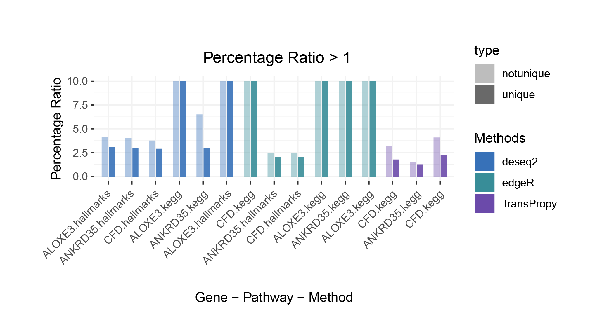
Percentage Ratio > 1

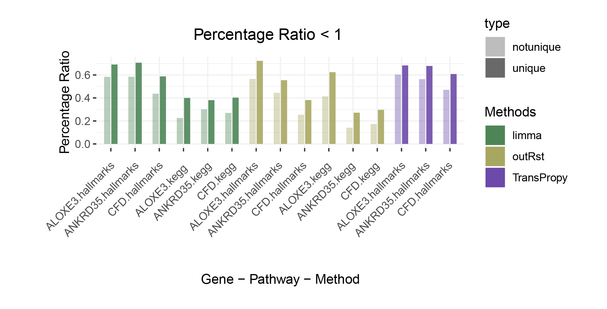
Percentage Ratio < 1

19.8

# Ensure percentage_ratio is numeric
final_data$percentage_ratio <- as.numeric(final_data$percentage_ratio)

# Split data based on 'type'
unique_df <- final_data[final_data$type == "unique", ]
notunique_df <- final_data[final_data$type == "notunique", ]

# Display unique Methods values
print("Unique Methods values for 'unique_df':")
print(unique(unique_df$Methods))

print("Unique Methods values for 'notunique_df':")
print(unique(notunique_df$Methods))


# Specify the order for Methods
method_order <- c("edgeR", "deseq2", "TransPropy", "limma", "outRst")

# Set factor levels for unique_df
unique_df$Methods <- factor(unique_df$Methods, levels = method_order)

# Set factor levels for notunique_df
notunique_df$Methods <- factor(notunique_df$Methods, levels = method_order)



# Create plotting function with significance stars and mean line
create_plot <- function(data, title, color_palette) {
  
  # Kruskal-Wallis test
  kruskal_res <- kruskal_test(data, percentage_ratio ~ Methods)
  
  # Pairwise Wilcoxon test
  pairwise_res <- data %>%
    pairwise_wilcox_test(
      percentage_ratio ~ Methods, 
      p.adjust.method = "bonferroni"
    )
  
  # Calculate means for each method
  means <- data %>%
    group_by(Methods) %>%
    summarise(mean = mean(percentage_ratio, na.rm = TRUE))
  
  # Plot
  p <- ggplot(data, aes(x = Methods, y = percentage_ratio, fill = Methods, color = Methods)) +
    geom_violin(alpha = 0.2, position = position_dodge(width = 0.75), size = 1) +
    geom_boxplot(width = 0.2, alpha = 0.5, position = position_dodge(width = 0.75), notch = FALSE, size = 1) +
    geom_point(shape = 21, size = 10, position = position_jitterdodge(dodge.width = 0), alpha = 0.5, color = "transparent") +
    geom_line(data = means, aes(x = Methods, y = mean, group = 1), 
              color = "#757575", linetype = 1, size = 5 , alpha = 0.5) +  # Add dashed line for means
    #geom_point(data = means, aes(x = Methods, y = mean, fill = Methods), shape = 21, size = 6) +  # Optional: add points for means
    scale_fill_manual(values = color_palette) +
    scale_color_manual(values = color_palette) +
    theme_bw() +
    labs(title = paste(title, "(Kruskal-Wallis p-value:", formatC(kruskal_res$p, format = "e", digits = 2), ")"),
         y = "Percentage Ratio") +
    theme(axis.text.x = element_text(angle = 45, hjust = 1))
  
  # Add significance stars based on Wilcoxon test results
  max_y <- max(data$percentage_ratio, na.rm = TRUE)
  comparisons <- combn(unique(data$Methods), 2, simplify = FALSE)
  y_positions <- seq(max_y + 1, by = 0.5, length.out = length(comparisons))  # Adjust spacing between significance stars
  
  # Add significance annotations
  x_value <- rep(1:4, 4:1)
  y_value <- rep(max(data$percentage_ratio), length(x_value)) + 1
  y_value <- y_value + c(0.5*1:4, 0.5*1:3, 0.5*1:2, 0.5)
  colors <- c("#388d98","#3771b8", "#6b4aaa","#4d8556","#a8a761" )
  color_value <- c(colors[2:5], colors[3:5], colors[4:5], colors[5])
  
  for (i in 1:nrow(pairwise_res)) {
    if (pairwise_res$p.adj.signif[i] != "ns") {
      y_tmp <- y_value[i]
      p <- p + annotate(geom = "text",
                        cex = 15,
                        label = pairwise_res$p.adj.signif[i],
                        x = x_value[i],
                        y = y_tmp,
                        color = color_value[i])
    }
  } 
  
  return(p)
}

# Define color palettes
hallmarks_colors <- c(
  "edgeR" = "#388d98",      
  "deseq2" = "#3771b8",     
  "TransPropy" = "#6b4aaa", 
  "limma" = "#4d8556",      
  "outRst" = "#a8a761"      
)

kegg_colors <- c(
  "edgeR" = "#388d98",      
  "deseq2" = "#3771b8",     
  "TransPropy" = "#6b4aaa", 
  "limma" = "#4d8556",      
  "outRst" = "#a8a761"      
)

# Check and adjust color palettes based on the data
unique_methods <- unique(unique_df$Methods)
notunique_methods <- unique(notunique_df$Methods)

# Filter palettes to match unique values
hallmarks_colors <- hallmarks_colors[names(hallmarks_colors) %in% unique_methods]
kegg_colors <- kegg_colors[names(kegg_colors) %in% notunique_methods]

# Create and display plots
plot_unique <- create_plot(unique_df, "Unique Types", hallmarks_colors)
plot_notunique <- create_plot(notunique_df, "Not Unique Types", kegg_colors)

# Display plots
print(plot_unique)
print(plot_notunique)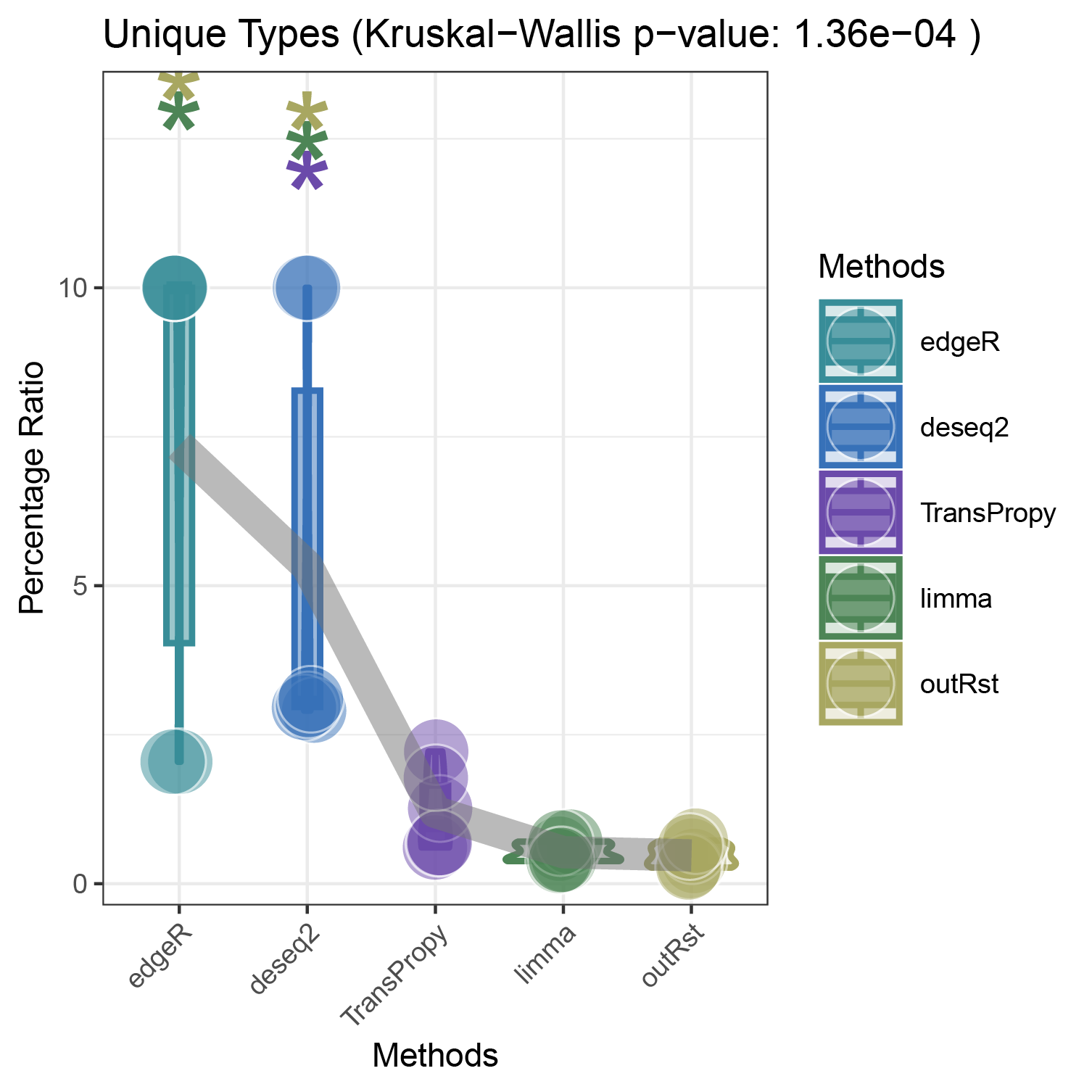

bar_violin_line_unique

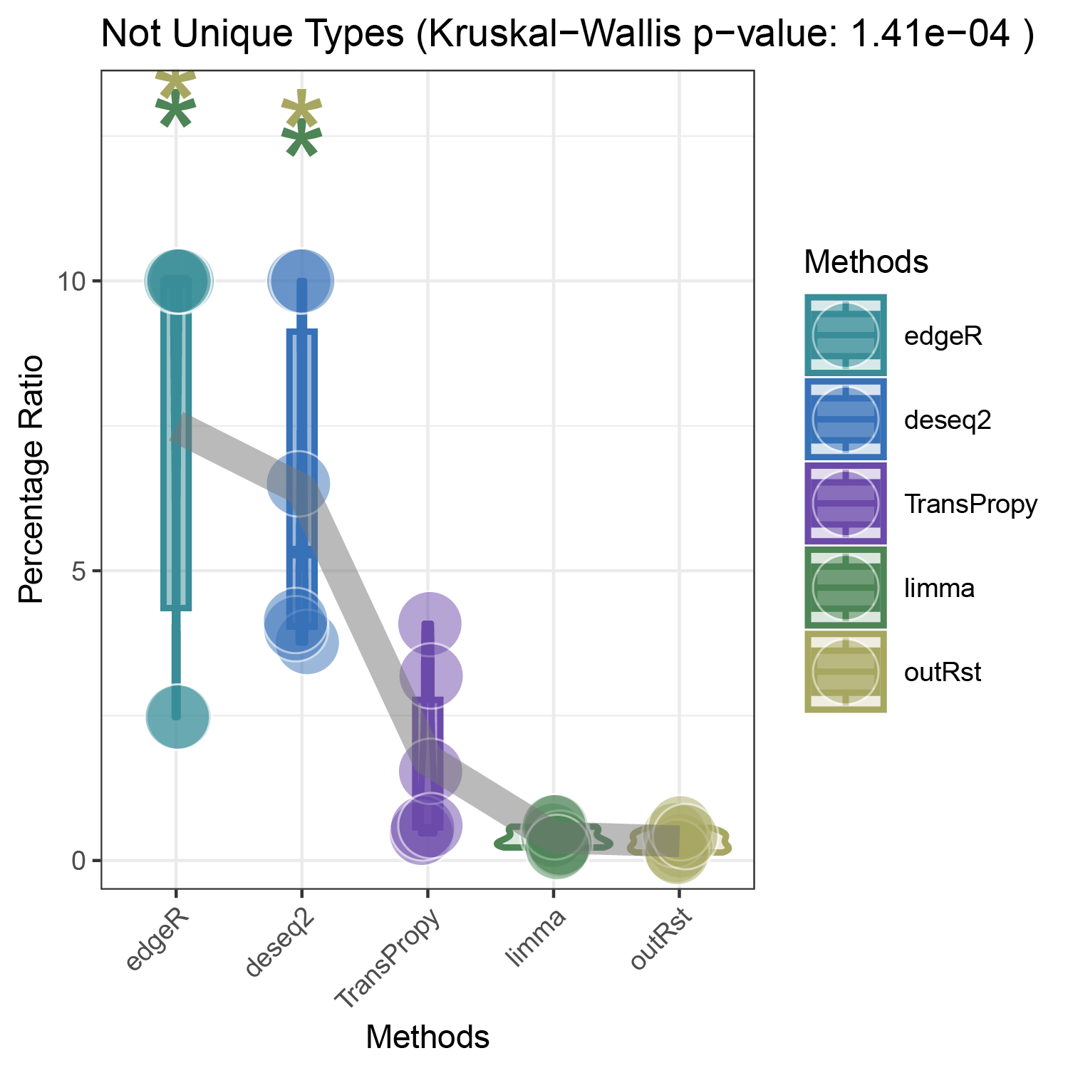
bar_violin_line_notunique

19.9 Methods

• Finding the top three genes with the highest countdown: CFD, ANKRD35, ALOXE3
• Count the number of core enrichment genes in the activated and inhibited pathways enriched under different genes (CFD, ANKRD35, ALOXE3), different pathway types, and different methods. This is done in two versions: unique (where all genes are deduplicated) and notunique (where the same gene appearing in different pathways is not deduplicated).

19.10 Discussion

All

The imbalance in the ratio of negative and positive genes observed in all unique groups (30 groups) will be further amplified in all notunique groups (30 groups). To understand this phenomenon, we conduct the following reasoning:

Since super core enrichment genes (those that repeatedly appear in different pathways) naturally play regulatory roles in more pathways, they tend to recur in the core enrichment gene statistics of all pathways. Now, let’s take a random example of a unique group and a notunique group. If the unique group consists entirely of ordinary core enrichment genes or super core enrichment genes, and each super core enrichment gene has the same repetition frequency, the final ratio will remain unchanged.

So, under what circumstances will the ratio disparity further amplify?

Taking the ratio of negative to positive genes greater than 0.5 as an example, both negative and positive genes have their own core enrichment and super core enrichment genes. The ratio will only further increase if the number or repetition degree of super core enrichment genes in negative genes is greater than that in positive genes. The ability to identify more super core enrichment genes or those with higher repetition frequencies (indicating greater importance) is the ideal goal of all algorithms, and this effect is consistently significant across all five algorithms.

deseq2/edgeR

The proportion of positively correlated genes is greater than that of negatively correlated genes (with some even having a ratio of 1), indicating a bias in the data results.

limma/outRst

In contrast to deseq2/edgeR, the proportion of positively correlated core genes is less than that of negatively correlated genes (with some ratios of positive to negative gene counts approaching 0).

TransPropy

The ratio of positively to negatively correlated gene counts lies between those of deseq2/edgeR and limma/outRst. As shown in the figure, TransPropy occupies the central position among the five methods, displaying a smooth transition trend, with most ratios approaching 0.5.（Better）